rss_ringoccs.diffrec.special_functions module¶

rss_ringoccs.diffrec.special_functions.compute_norm_eq(w_func, error_check=True)¶

Purpose:

Compute normalized equivalenth width of a given function.

Arguments:

w_func (np.ndarray):
	Function with which to compute the normalized equivalent width of.

Outputs:

normeq (float):	The normalized equivalent width of w_func.

Notes:

The normalized equivalent width is effectively computed using Riemann sums to approximate integrals. Therefore large dx values (Spacing between points in w_func) will result in an inaccurate normeq. One should keep this in mind during calculations.

Examples:

Compute the Kaiser-Bessel 2.5 window of width 30 and spacing 0.1, and then use compute_norm_eq to compute the normalized equivalent width:

>>> from rss_ringoccs import diffrec as dc
>>> w = dc.window_functions.kb25(30, 0.1)
>>> normeq = dc.special_functions.compute_norm_eq(w)
>>> print(normeq)
1.6573619266424229

In contrast, the actual value is 1.6519208. Compute the normalized equivalent width for the squared cosine window of width 10 and spacing 0.25.

>>> from rss_ringoccs import diffrec as dc
>>> w = dc.window_functions.coss(10, 0.25)
>>> normeq = dc.special_functions.compute_norm_eq(w)
>>> print(normeq)
1.5375000000000003

The normalized equivalent width of the squared cosine function can be computed exactly using standard methods from a calculus course. It’s value is exactly 1.5 If we use a smaller dx when computing w, we get a better approximation. Use width 10 and spacing 0.001.

>>> from rss_ringoccs import diffrec as dc
>>> w = dc.window_functions.coss(10, 0.001)
>>> normeq = dc.special_functions.compute_norm_eq(w)
>>> print(normeq)
1.50015

rss_ringoccs.diffrec.special_functions.d2psi(kD, r, r0, phi, phi0, B, D)¶

Purpose:

Compute $\mathrm{d}^2\psi/\mathrm{d}\phi^2$

Arguments:

r0 (np.ndarray):
kD (float):	Wavenumber, unitless.
r (float):	Radius of reconstructed point, in kilometers.
	Radius of region within window, in kilometers.
phi (np.ndarray):
	Root values of $\mathrm{d}\psi/\mathrm{d}\phi$ , radians.
phi0 (np.ndarray):
	Ring azimuth angle corresponding to r0, radians.
B (float):	Ring opening angle, in radians.
D (float):	Spacecraft-RIP distance, in kilometers.

Outputs:

dpsi (np.ndarray):
	Second partial derivative of $\psi$ with respect to $\phi$ .

rss_ringoccs.diffrec.special_functions.double_slit_diffraction(x, z, a, d)¶

Purpose:

Compute diffraction through a double slit for the variable x with a distance z from the slit and slit parameter a and a distance d between the slits. This assumes Fraunhofer diffraction.

Variables:

x:	A real or complex argument, or numpy array.
z (float):	The perpendicular distance from the slit plane to the observer.
a (float):	The slit parameter. This is a unitless paramter defined as the ratio between the slit width and the wavelength of the incoming signal.
d (float):	The distance between slits.

Outputs:

f:	Single slit diffraction pattern.

rss_ringoccs.diffrec.special_functions.dpsi(kD, r, r0, phi, phi0, B, D)¶

Purpose:

Compute $\mathrm{d}\psi/\mathrm{d}\phi$

Arguments:

r0 (np.ndarray):
kD (float):	Wavenumber, unitless.
r (float):	Radius of reconstructed point, in kilometers.
	Radius of region within window, in kilometers.
phi (np.ndarray):
	Root values of $\mathrm{d}\psi/\mathrm{d}\phi$ , radians.
phi0 (np.ndarray):
	Ring azimuth angle corresponding to r0, radians.
B (float):	Ring opening angle, in radians.
D (float):	Spacecraft-RIP distance, in kilometers.

Outputs:

dpsi (array):	Partial derivative of $\psi$ with respect to $\phi$ .

rss_ringoccs.diffrec.special_functions.dpsi_ellipse(kD, r, r0, phi, phi0, B, D, ecc, peri)¶

Purpose:

Compute $\mathrm{d}\psi/\mathrm{d}\phi$

Arguments:

r0 (np.ndarray):
kD (float):	Wavenumber, unitless.
r (float):	Radius of reconstructed point, in kilometers.
	Radius of region within window, in kilometers.
phi (np.ndarray):
	Root values of $\mathrm{d}\psi/\mathrm{d}\phi$ , radians.
phi0 (np.ndarray):
	Ring azimuth angle corresponding to r0, radians.
B (float):	Ring opening angle, in radians.
D (float):	Spacecraft-RIP distance, in kilometers.

Outputs:

dpsi (array):	Partial derivative of $\psi$ with respect to $\phi$ .

rss_ringoccs.diffrec.special_functions.fresnel_cos(x)¶

Purpose:

Compute the Fresnel cosine function.

Arguments:

x (np.ndarray or float):
	A real or complex number, or numpy array.

Outputs:

f_cos (np.ndarray or float):
	The fresnel cosine integral of x.

Notes:

The Fresnel Cosine integral is the solution to the equation 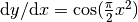$\mathrm{d}y/\mathrm{d}x = \cos(\frac\pi 2 x^2)$ , $y(0) = 0$ . In other words, $y = \int_{t=0}^{x}\cos(\frac\pi 2 t^2)\mathrm{d}t$
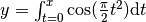
The Fresnel Cosine and Sine integrals are computed by using the scipy.special Error Function. The Error Function, usually denoted Erf(x), is the solution to $\mathrm{d}y/\mathrm{d}x = \frac{2}{\sqrt{\pi}}\exp(-x^2)$ , $y(0) = 0$ . That is: $y = \frac{2}{\sqrt{\pi}}\int_{t=0}^{x}\exp(-t^2)\mathrm{d}t$ . Using Euler’s Formula for exponentials allows one to use this to solve for the Fresnel Cosine integral.
The Fresnel Cosine integral is used for the solution of diffraction through a square well. Because of this it is useful for forward modeling problems in radiative transfer and diffraction.

Examples:

Compute and plot the Fresnel Cosine integral.

>>> import rss_ringoccs.diffcorr.special_functions as sf
>>> import numpy as np
>>> import matplotlib.pyplot as plt
>>> x = np.array(range(0,10001))*0.01 - 50.0
>>> y = sf.fresnel_cos(x)
>>> plt.show(plt.plot(x,y))

rss_ringoccs.diffrec.special_functions.fresnel_scale(Lambda, d, phi, b, deg=False)¶

Purpose:

Compute the Fresnel Scale from $\lambda$ , $D$ , $\phi$ , and $B$ .

Arguments:

Lambda (np.ndarray or float):
	Wavelength of the incoming signal.
d (np.ndarray or float):
	RIP-Spacecraft Distance.
phi (np.ndarray or float):
	Ring azimuth angle.
b (np.ndarray or float):
	Ring opening angle.

Keywords:

deg (bool):	Set True if $\phi$ or $B$ are in degrees. Default is radians.

Output:

fres (np.ndarray or float):
	The Fresnel scale.

Note:

$\lambda$ and $D$ must be in the same units. The output (Fresnel scale) will have the same units as $\lambda$ and d. In addition, $B$ and $\phi$ must also have the same units. If $B$ and $\phi$ are in degrees, make sure to set deg=True. Default is radians.

rss_ringoccs.diffrec.special_functions.fresnel_sin(x)¶

Purpose:

Compute the Fresnel sine function.

Variables:

x (np.ndarray or float):
	The independent variable.

Outputs:

f_sin (np.ndarray or float):
	The fresnel sine integral of x.

Notes:

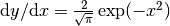
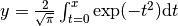
The Fresnel sine integral is the solution to the equation $\mathrm{d}y/\mathrm{d}x = \sin(\frac\pi 2 x^2)$ , $y(0) = 0$ . In other words, $y = \int_{t=0}^{x}\sin(\frac\pi 2 t^2) dt$
The Fresnel Cossine and Sine integrals are computed by using the scipy.special Error Function. The Error Function, usually denoted Erf(x), is the solution to $\mathrm{d}y/\mathrm{d}x = \frac{2}{\sqrt{\pi}} \exp(-x^2)$ , $y(0) = 0$ . That is: $y = \frac{2}{\sqrt{\pi}}\int_{t=0}^{x}\exp(-t^2)dt$ . Using Euler’s Formula for exponentials allows one to use this to solve for the Fresnel Sine integral.
The Fresnel sine integral is used for the solution of diffraction through a square well. Because of this is is useful for forward modeling problems in radiative transfer and diffraction.

Examples:

Compute and plot the Fresnel Sine integral.

>>> import rss_ringoccs.diffcorr.special_functions as sf
>>> import numpy as np
>>> import matplotlib.pyplot as plt
>>> x = np.array(range(0,10001))*0.01 - 50.0
>>> y = sf.fresnel_sin(x)
>>> plt.show(plt.plot(x,y))

rss_ringoccs.diffrec.special_functions.inverse_square_well_diffraction(x, a, b, F)¶

rss_ringoccs.diffrec.special_functions.psi(kD, r, r0, phi, phi0, B, D)¶

Purpose:

Compute $\psi$ (MTR Equation 4)

Arguments:

r0 (np.ndarray):
kD (float):	Wavenumber, unitless.
r (float):	Radius of reconstructed point, in kilometers.
	Radius of region within window, in kilometers.
phi (np.ndarray):
	Root values of $\mathrm{d}\psi/\mathrm{d}\phi$ , radians.
phi0 (np.ndarray):
	Ring azimuth angle corresponding to r0, radians.
B (float):	Ring opening angle, in radians.
D (float):	Spacecraft-RIP distance, in kilometers.

Outputs:

psi (np.ndarray):
	Geometric Function from Fresnel Kernel.

rss_ringoccs.diffrec.special_functions.resolution_inverse(x)¶

Purpose:

Compute the inverse of $y = x/(\exp(-x)+x-1)$

Arguments:

x (np.ndarray or float):
	Independent variable

Outputs:

f (np.ndarray or float):
	The inverse of $x/(\exp(-x)+x-1)$

Dependencies:

numpy
scipy.special

Method:

The inverse of $x/(\exp(-x)+x-1)$ is computed using the LambertW function. This function is the inverse of $y = x\exp(x)$ . This is computed using the scipy.special subpackage using their lambertw function.

Warnings:

The real part of the argument must be greater than 1.
The scipy.special lambertw function is slightly inaccurate when it’s argument is near $-1/e$ . This argument is $z = \exp(x/(1-x)) * x/(1-x)$

Examples:

Plot the function on the interval (1,2)

>>> import rss_ringoccs.diffcorr.special_functions as sf
>>> import numpy as np
>>> x = np.array(range(0,1001))*0.001+1.01
>>> y = sf.resolution_inverse(x)
>>> import matplotlib.pyplot as plt
>>> plt.show(plt.plot(x,y))

rss_ringoccs.diffrec.special_functions.savitzky_golay(y, window_size, order, deriv=0, rate=1)¶

Purpose:

To smooth data with a Savitzky-Golay filter. This removes high frequency noise while maintaining many of the original features of the input data.

Arguments:

window_size (int):
y (np.ndarray):	The input “Noisy” data.
	The length of the window. Must be an odd number.
order (int):	The order of the polynomial used for filtering. Must be less then window_size - 1.

Keywords:

deriv (int):	The order of the derivative what will be computed.

Output:

y_smooth (np.ndarray):
	The data smoothed by the Savitzky-Golay filter. This returns the nth derivative if the deriv keyword has been set.

Notes:

The Savitzky-Golay is a type of low-pass filter, particularly suited for smoothing noisy data. The main idea behind this approach is to make for each point a least-square fit with a polynomial of high order over a odd-sized window centered at the point.

rss_ringoccs.diffrec.special_functions.single_slit_diffraction(x, z, a)¶

Purpose:

Compute diffraction through a single slit for the variable x with a distance z from the slit and slit parameter a. This assume Fraunhofer diffraction.

Variables:

x:	A real or complex argument, or numpy array.
z (float):	The perpendicular distance from the slit plane to the observer.
a (float):	The slit parameter. This is a unitless paramter defined as the ratio between the slit width and the wavelength of the incoming signal.

Outputs:

f:	Single slit diffraction pattern.

rss_ringoccs.diffrec.special_functions.square_well_diffraction(x, a, b, F)¶